Topological relations

Quick recap: vector data

• In GIScience and Geodatabases, you learned about the Simple Features standard (ISO 19125)
• Features = geometry (point, line, polygon) + attributes (columns)
• In R: sf objects are data frames with a geometry column

• So far, we’ve worked with features mostly in isolation — reading, plotting, transforming
• But often we need to ask: how do two features relate to each other spatially?
  • Does this river flow through this canton?
  • Which bus stops are within this district?
• This is where topological relations come in

Named topological relations

• Topological relations describe the spatial relationships between objects
• Also called binary topological relationships or binary predicates
• Logical statements (TRUE/FALSE) about two objects
• The two objects are defined by ordered sets of points (typically forming points, lines and polygons) in two or more dimensions (Egenhofer and Herring 1990)

Usage

• Topological relations can be used to subset or join spatial data
• For example:
  • Subsetting: Return all rivers that flow through the canton of Zurich
  • Joining: For every train station, give me the name of the municipality it lies within

Common predicates in sf

• Most GIS software offers common topological relations as functions
• sf provides many: st_intersects(), st_disjoint(), st_touches(), st_crosses(), …
• Each works slightly differently and fits different contexts
• Examples:
  • st_covers(x, y) → TRUE if no points of x are outside y
  • st_touches(x, y) → TRUE if geometries share boundary points but interiors don’t intersect

Key predicates visualized

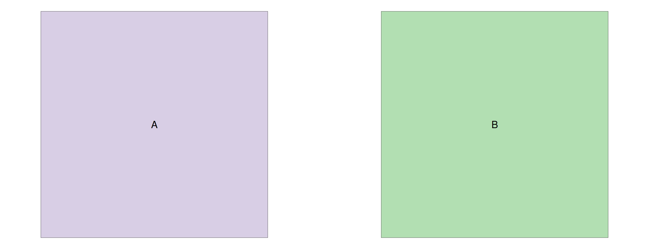
(a) st_disjoint: no shared points

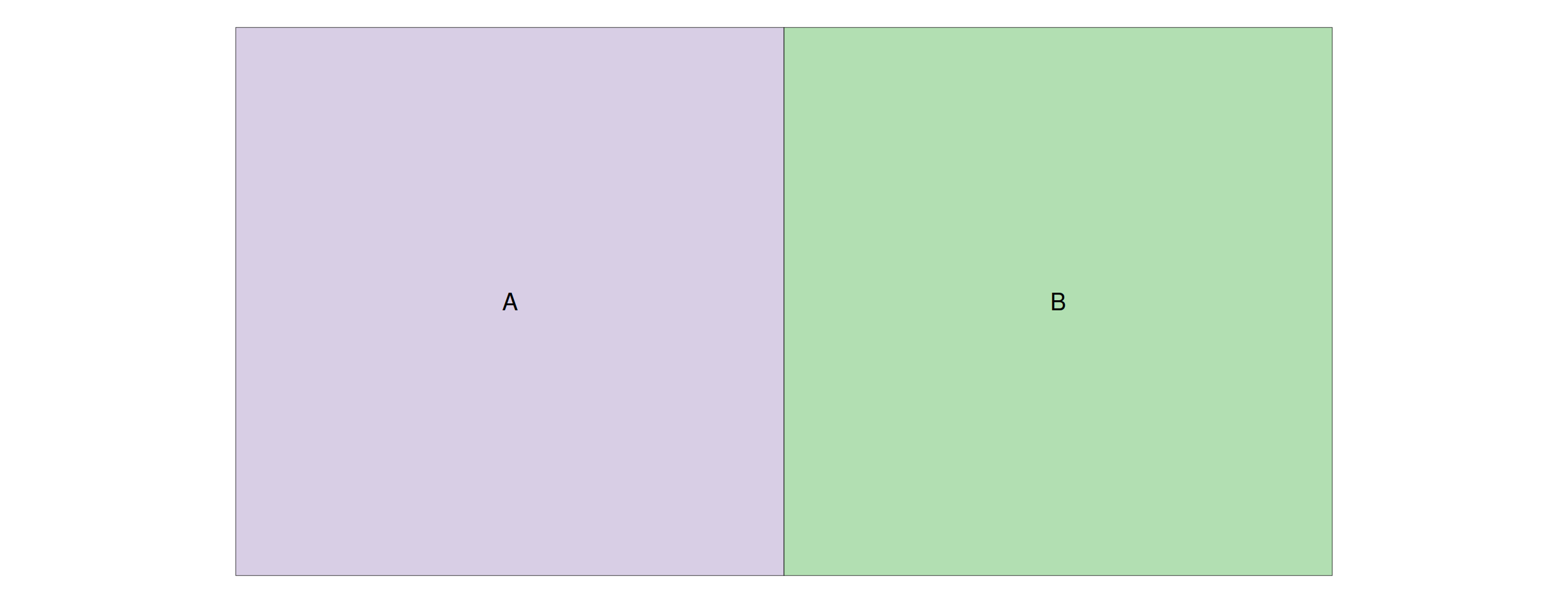
(b) st_touches: shared boundary only

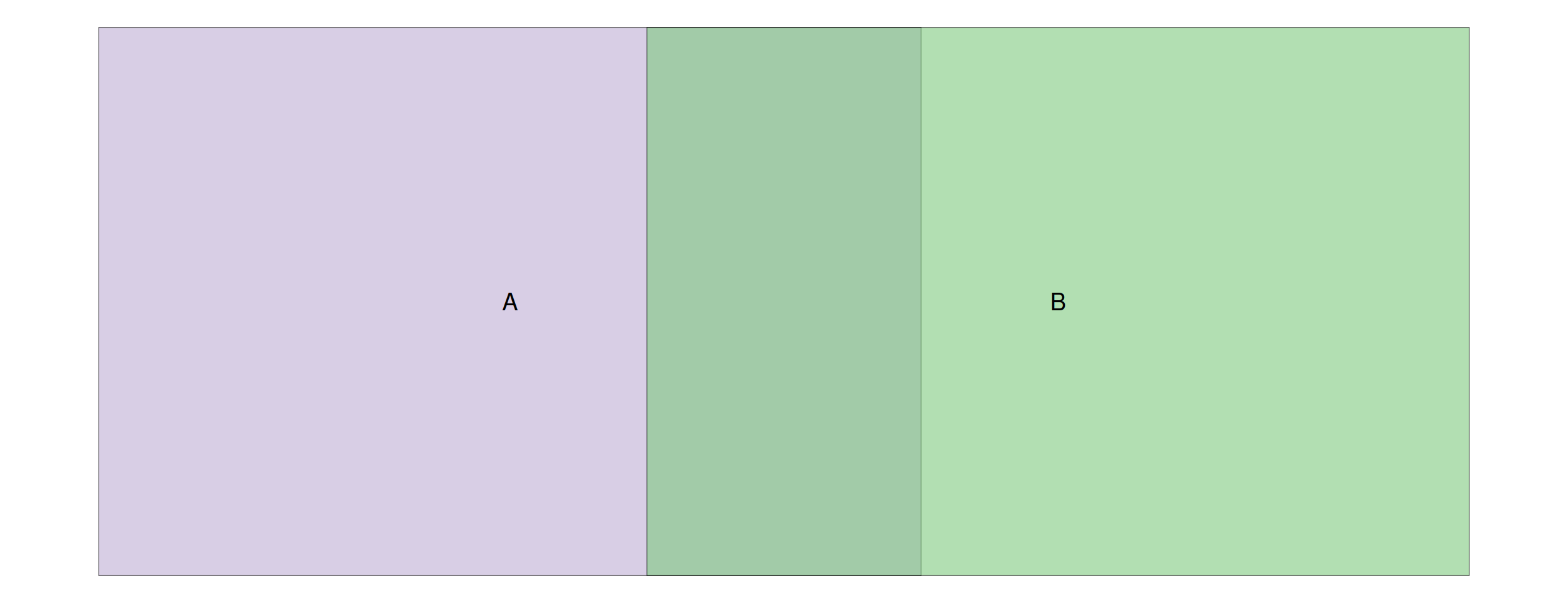
(c) st_intersects: any shared points (here with overlap)

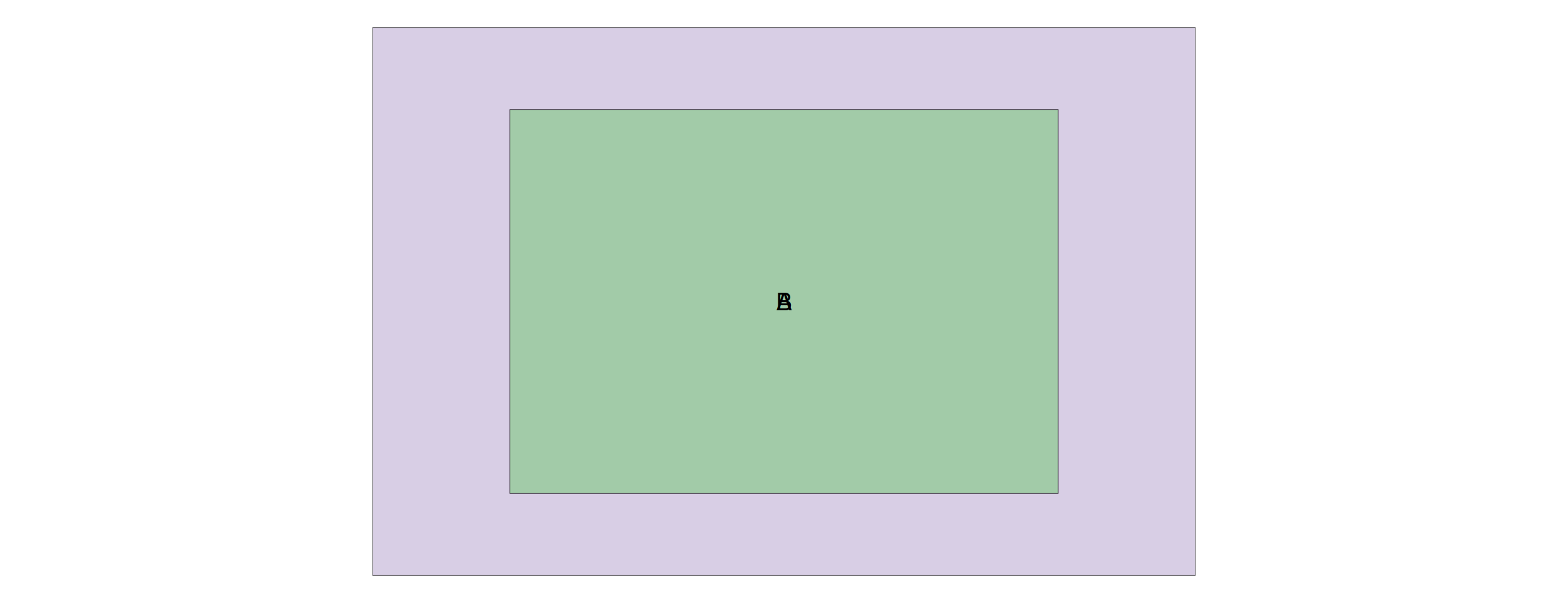
(d) st_contains: B entirely within A

Figure 1: Key topological relations between two polygons (A in purple, B in green)

Symmetry and order

• Some relations are symmetrical (order doesn’t matter)
  • st_touches(x, y) = st_touches(y, x)
• Others are asymmetrical (order matters!)
  • st_contains(x, y) ≠ st_contains(y, x)
• Some require extra arguments
  • st_is_within_distance() needs a dist argument
• Full list: ?geos_binary_pred

Predicates vs. operations

Don’t confuse predicates with operations!

• Predicate (e.g. st_intersects): “Do these geometries intersect?” → returns TRUE/FALSE
• Operation (e.g. st_intersection): “Give me the geometry where they overlap” → returns a new geometry

The same naming pattern applies to other pairs: st_difference (operation) has no corresponding predicate, while st_touches (predicate) has no corresponding operation.

Predicate return types

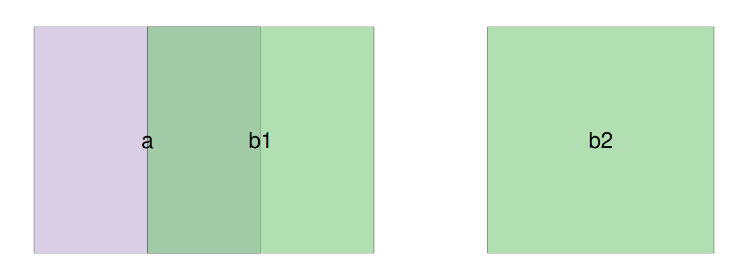
Figure 2: Polygon a (purple) overlaps b1 but is disjoint from b2

• st_intersects(x, y) does not return a simple TRUE/FALSE vector
• Returns a sparse geometry binary predicate (sgbp) — a list of matching indices

st_intersects(a, b)
## Sparse geometry binary predicate list of length 1, where the predicate
## was `intersects'
##  1: 1

• lengths() counts the number of matches per feature
• Use sparse = FALSE to get a dense logical matrix instead

st_intersects(a, b, sparse = FALSE)
##      [,1]  [,2]
## [1,] TRUE FALSE

Applying predicates: subsetting

Now that we know how predicates work, let’s use them to subset and join spatial data.

Spatial subsetting

• Predicates can be used to subset one dataset based on another
• Example data: playgrounds, public transport stops, and Stadtkreise in Zurich

library(sf)
library(readr)

# source: https://www.stadt-zuerich.ch/geodaten/
playgrounds <- read_sf("data/vector-deepdive/playgrounds.gpkg")
publictransport <- read_sf("data/vector-deepdive/public_transport.gpkg")
kreise <- read_sf("data/vector-deepdive/stadtkreise-zh.gpkg")

• Default predicate: st_intersects
• Example: which playgrounds lie within Stadtkreis 1?

kreis1 <- kreise[kreise$STADTKREIS == "Kreis 1", ]

playgrounds_k1 <- playgrounds[kreis1, ]  # st_intersects is the default

nrow(playgrounds_k1)
## [1] 6

Distance-based subsetting

• Not limited to topological predicates — can also use distance-based ones
• Example: which playgrounds are within 100m of a public transport stop?

# Using the shorthand notation
playgrounds_close <- playgrounds[publictransport,,op = st_is_within_distance, dist = 100]

Same thing, more readable with st_filter():

playgrounds_close <- st_filter(playgrounds, publictransport, .predicate = st_is_within_distance, dist = 100)

Figure 3: Note that the playgrounds within 100m of public transport (red dots) are a subset of all the playgrounds

From subsetting to joining

Subsetting filters features — what if we want to transfer attributes instead?

Spatial joins

• Joins transfer attributes from one dataset to another based on spatial relationship
• st_join(x, y): for each feature in x, find matching features in y and attach their columns
• Example: add the name of the nearest public transport stop to each playground

st_nearest_feature is not strictly a binary predicate, but is very useful for spatial joins. To make the example clearer, we first discard all unnecessary columns from the datasets.

publictransport <- publictransport[,"CHSTNAME"]

playgrounds <- playgrounds[, "name"]


playgrounds_join <- st_join(
  playgrounds, 
  publictransport, 
  join = st_nearest_feature
  )

playgrounds_join

Simple feature collection with 184 features and 2 fields
Geometry type: POINT
Dimension:     XY
Bounding box:  xmin: 2677632 ymin: 1242927 xmax: 2687639 ymax: 1253914
Projected CRS: CH1903+ / LV95
# A tibble: 184 × 3
   name                                                    geom CHSTNAME        
 * <chr>                                            <POINT [m]> <chr>           
 1 Buchenweg                                  (2685485 1245793) Zürich, Burgwies
 2 Buchlern Sportanlage                       (2678406 1248303) Zürich, Friedho…
 3 Mobile Spielanimation PAZMobile Spielanim… (2682898 1244212) Zürich, Rote Fa…
 4 Alfred-Altherr-Terrasse                    (2684082 1249963) Zürich, Langens…
 5 Auf der Egg                                (2682672 1243867) Zürich, Kalchbü…
 6 Belvoirpark                                (2682665 1245835) Zürich, Brunaus…
 7 Josefswiese                                (2681846 1248909) Zürich, Schiffb…
 8 Gertrudplatz                               (2681431 1247583) Zürich, Locherg…
 9 Wahlenpark                                 (2683172 1252246) Zürich, Max-Bil…
10 Rote Fabrik                                (2683004 1244150) Zürich, Rote Fa…
# ℹ 174 more rows

Join cardinality

• playgrounds_join has the same rows as playgrounds + extra column CHSTNAME
  • Why? Each playground has exactly one nearest station
• But row count can change with other join predicates!
  • Within 100m: a playground may match zero or multiple stops

playgrounds_join2 <- st_join(
  playgrounds, 
  publictransport, 
  join = st_is_within_distance, 
  dist = 100
  )

nrow(playgrounds)
## [1] 184

nrow(playgrounds_join2)
## [1] 186

playgrounds_join2

Simple feature collection with 186 features and 2 fields
Geometry type: POINT
Dimension:     XY
Bounding box:  xmin: 2677632 ymin: 1242927 xmax: 2687639 ymax: 1253914
Projected CRS: CH1903+ / LV95
# A tibble: 186 × 3
   name                                                    geom CHSTNAME        
 * <chr>                                            <POINT [m]> <chr>           
 1 Buchenweg                                  (2685485 1245793) <NA>            
 2 Buchlern Sportanlage                       (2678406 1248303) <NA>            
 3 Mobile Spielanimation PAZMobile Spielanim… (2682898 1244212) Zürich, Rote Fa…
 4 Alfred-Altherr-Terrasse                    (2684082 1249963) <NA>            
 5 Auf der Egg                                (2682672 1243867) Zürich, Kalchbü…
 6 Belvoirpark                                (2682665 1245835) <NA>            
 7 Josefswiese                                (2681846 1248909) <NA>            
 8 Gertrudplatz                               (2681431 1247583) <NA>            
 9 Wahlenpark                                 (2683172 1252246) <NA>            
10 Rote Fabrik                                (2683004 1244150) Zürich, Rote Fa…
# ℹ 176 more rows

Join order

• Order matters (just like regular joins)
• st_join = left join by default
• Result keeps the geometry of the left dataset

kreise <- kreise[,"STADTKREIS"]

publictransport_join <- st_join(publictransport, kreise)

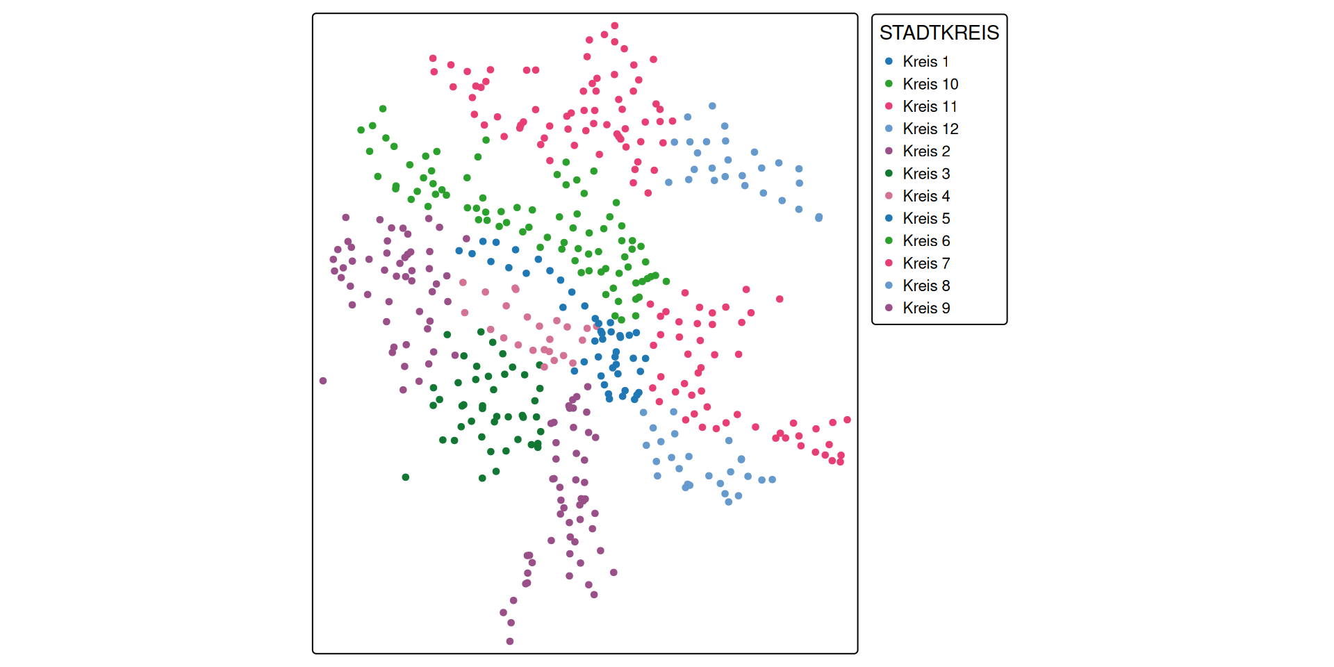
• Reverse order → each stadtkreis gets duplicated for every intersecting point

kreise_join <- st_join(kreise, publictransport)

nrow(kreise)
## [1] 12

nrow(kreise_join)
## [1] 477

(a) Dataset kreise with 12 features

(b) Dataset kreise_join with 477 features

Figure 4: Note that all the duplicate stadtkreise overlap each other, so when you visualize the data, the issue is not noticeable

Summary

Task	Function	Key arguments
Test a relationship	st_intersects(), st_covers(), …	sparse = FALSE for logical matrix
Subset by predicate	x[y, ] or st_filter()	op / .predicate, dist
Join by predicate	st_join(x, y)	join, left = TRUE

• Default predicate is always st_intersects
• Prefer st_covers over st_contains for point-in-polygon
• Join order determines geometry and potential row duplication

Custom topological relations

A motivating problem

• Consider a 3×3 chessboard (Figure 5)
• Which fields share a full edge with the origin? (like a rook’s move)
• st_touches won’t work — it also matches diagonal neighbours (shared point)
• We need a way to express: “shared boundary must be a line, not just a point”

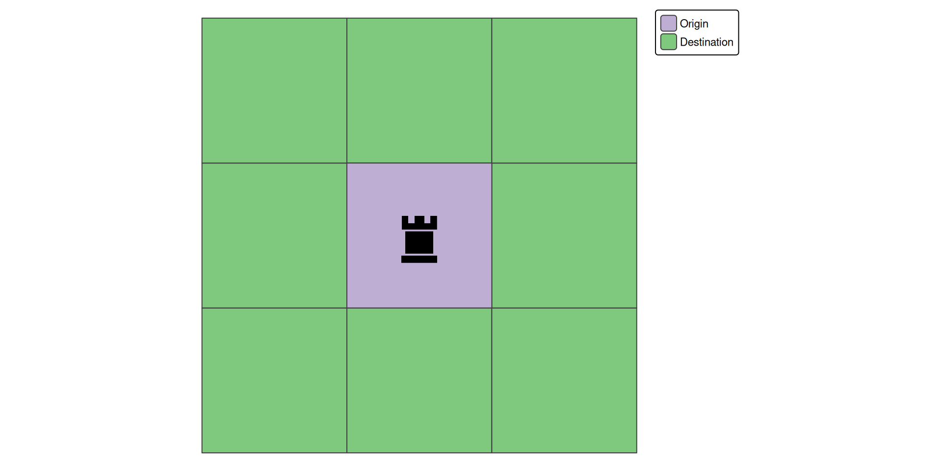
Figure 5: A 3x3 chessboard with a rook in the center field (origin). Which fields can the rook reach, if the constraint is that the destination field need to share an edge with the origin?

The DE-9IM

• DE-9IM (Dimensionally Extended nine-Intersection Model) gives fine-grained control
• DE-9IM is the formal model behind all named predicates
• Describes the relationship as a 3×3 matrix: interior, boundary, exterior of each geometry
• Table 1 shows the analysis for two overlapping polygons

Table 1: DE-9IM for two edge-sharing squares (A in purple, B in green). Red shading/line = intersection result.

	Interior (B)	Boundary (B)	Exterior (B)
Interior (A)
Boundary (A)
Exterior (A)

Table 2: The DE-9IM for the rooks case. This can be flattend into the string F***1****

	Interior	Boundary	Exterior
Interior	F	*	*
Boundary	*	1	*
Exterior	*	*	*

• Each cell shows the intersection of a part of A (row) with a part of B (column)
• For the rook, we only care about two cells:
  • Interior ∩ Interior = F (no overlap)
  • Boundary ∩ Boundary = 1 (shared edge = a line, not just a point)
• Everything else = * (don’t care)
• Flatten row by row into the pattern → F***1****

This is what distinguishes edge-sharing (rook) from corner-sharing (bishop) neighbours: for a bishop, Boundary ∩ Boundary = 0 (a point), while for the rook it must be 1 (a line). The encoding is: F = empty, 0 = point, 1 = line, 2 = area. * means “any value” and T means “any non-empty value” (i.e. 0, 1, or 2).

Predicates as patterns

• Every named predicate = one or more DE-9IM patterns

Predicate	DE-9IM pattern(s)
st_intersects	T********, *T*******, ***T*****, ****T**** (any non-empty intersection)
st_touches	FT*******, F**T*****, F***T****
st_contains	T*****FF*
st_within	T*F**F***

• st_contains and st_within are mirror images (swap rows ↔︎ columns)
• * = wildcard, matches F, 0, 1, or 2

• The exact values 0, 1, 2 describe the dimension of the intersection (point, line, area).
• In patterns, T means “any non-empty intersection” - i.e. it matches 0, 1, or 2 but not F.
• So T is used when you care that something intersects but don’t care how (point vs line vs area), while 0/1/2 pin down the exact dimension.

Create a custom st_rook function and use it like any named predicate:

st_rook <- \(x, y) st_relate(x, y, pattern = "F***1****")

grid_rook <- grid_dest[grid_orig, , op = st_rook] |> 
  st_sample(1000, type = "hexagonal",by_polygon = TRUE)

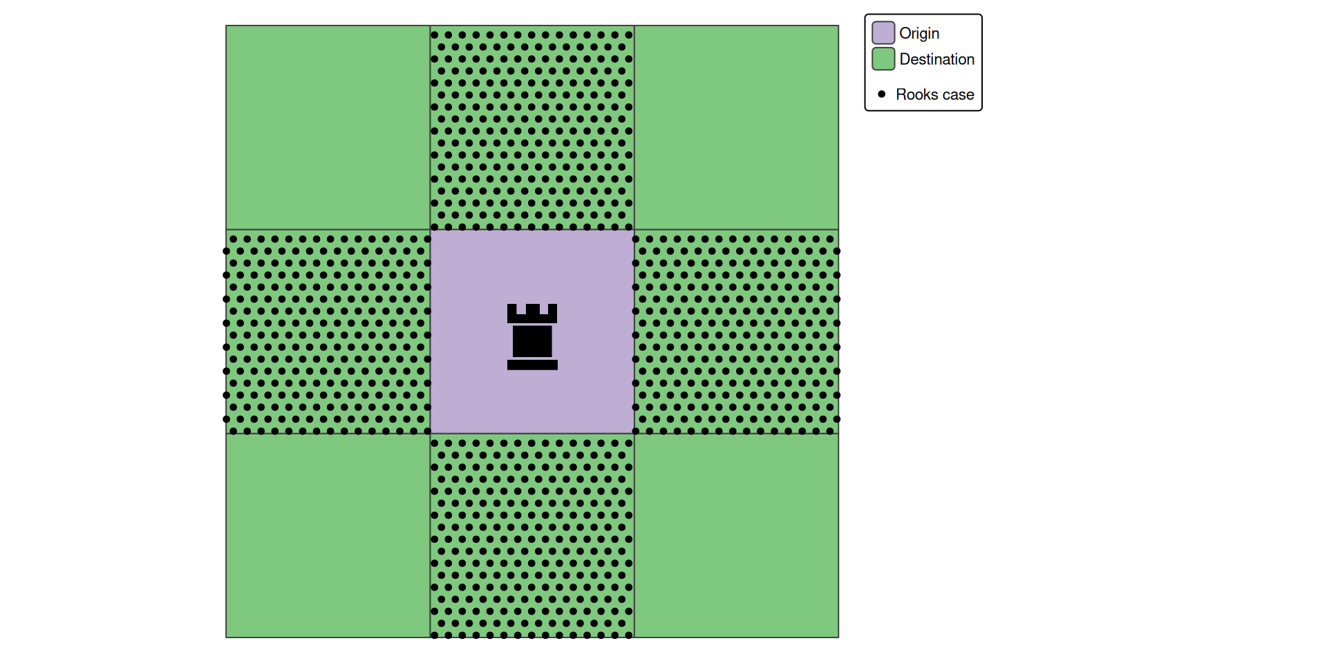
Figure 6: The chessboard situation with the potential fields for the rook highlighted with a red outline

Wrap-up

• Named predicates (st_intersects, st_covers, …) cover most use cases for subsetting and joining
• When they don’t suffice, DE-9IM patterns let you define custom relations (st_relate)
• Key pitfalls to remember:
  • st_contains vs st_covers (boundary matters!)
  • Join order determines geometry and row count
  • Predicates return sparse index lists, not logical vectors (use sparse = FALSE if needed)

References

Egenhofer, Max, and John Herring. 1990. “A Mathematical Framework for the Definition of Topological Relations.” Proc. The Fourth International Symposium on Spatial Data Handing, 803–13.