Raster data on disk

Spatiotemporal Data Science · FS26

Today

1. GDAL CLI — what it is, when to use it, how commands are structured
2. Raster data types — choosing the right type, rescaling, scale/offset
3. gdal raster info — inspecting raster files from the terminal
4. NoData — how missing values are stored on disk
5. Categorical rasters — integer encoding + attribute tables
6. Compression — lossless compression with gdal raster convert
7. Reprojection — changing CRS with gdal raster reproject

GDAL CLI

GDAL CLI

• GDAL is the basis for most GIS software — we can also call it directly from the terminal
• Ships several raster programs, each designed for a specific task
• Advantages over R / Python: faster, memory-efficient, composable, portable
• Install via conda:

conda install -c conda-forge gdal

• We’ve already used GDAL indirectly: terra, QGIS, and many other tools call it under the hood
• “Block-by-block” means GDAL reads and writes in tiles — a 10GB raster can be processed with <1MB RAM
• In practice: use CLI for data prep / inspection, R/Python for analysis and visualization

When does GDAL CLI shine?

• Reprojection: Block-by-block — no full load into RAM → fast!
• Format conversion: no full load into RAM → fast!
• Extracting file info: Instant, no environment startup — great for quick access
• Batch processing: One shell loop over hundreds of files; no memory accumulation
• Mosaicking: Combining hundreds of tiles stays out of RAM entirely
• Building overviews: Purely structural file operation
• Pipelines / CI: Slots into shell scripts, Makefiles, CI/CD without an R/Python runtime

• Reprojection and batch processing are the two most commonly cited by practitioners
• “No environment startup” matters a lot in scripts: starting R just to run gdalinfo on 1000 files adds minutes of overhead
• Overviews (pyramids) allow fast display at lower resolutions — QGIS and other tools use them automatically
• We’ll have a look at reprojection and file info extraction

Which CLI tools do you already use?

• conda — manage environments and packages
• pip — install Python packages
• git — version control

• Ask students to raise their hand for each one — most will have used at least 3
• The point: they’re already CLI users; GDAL is not a new paradigm, just a new tool
• Some may also use ssh, jupyter, docker — worth asking

Anatomy of a CLI call

program    subcommand    flag  flag-value     argument
   ↓           ↓          ↓       ↓             ↓
conda     install         -c   conda-forge     gdal
⎺⎺⎺     ⎺⎺⎺⎺⎺       ⎺⎺  ⎺⎺⎺⎺⎺⎺⎺     ⎺⎺

• Program — the tool being called
• Subcommand — the action to perform (not all tools have these)
• Flag — modifies behaviour; -c is shorthand for --channel
• Flag value — the value passed to a flag
• Argument — positional value the command operates on (no - prefix)

• Short flags (-c) and long flags (--channel) are equivalent; long flags are more readable in scripts
• Flags can appear in any order; arguments are positional (order matters)
• This anatomy applies to every CLI tool: git commit -m "message", quarto render --to pdf, gdal raster info -f json file.tif

New GDAL API

• Prior to GDAL 3.11, the suite of GDAL programs had a highly inconsistent API
• With 3.11, GDAL introduced a unified CLI entry point — gdal <noun> <verb>
• The new API is great, but WIP
• Our examples use the new API
• See webinar GDAL Command Line Interface Modernization

Task	Old API	New API (3.11+)
Inspect	gdalinfo	gdal raster info
Convert	gdal_translate	gdal raster convert
Reproject	gdalwarp	gdal raster reproject

• You will see the old API in the wild — documentation, Stack Overflow answers often still use it
• The old tools are not deprecated; new API is additive
• Check your version: gdal --version

Input → output

GDAL is non-destructive by design — it always reads from a source and writes to a new destination:

gdal raster reproject --dst-crs EPSG:2056 input.tif output.tif
                                           ─────────  ──────────
                                           source     new file, never touches source

• The original file is never modified
• Every operation requires both <input> and <output> arguments
• Consequence: you need roughly 2× the disk space during processing

Exception: gdal edit — metadata-only changes (CRS, NoData, scale/offset) can be applied in place

• Non-destructive is safer: if something goes wrong, the original is intact
• gdal edit is useful when you just need to assign a missing CRS or fix a NoData flag without rewriting the full file
• In pipelines, the output of one step becomes the input of the next — plan your disk usage accordingly

Raster data types

Raster data types

• Raster data on disk is always stored as numeric (no strings, no factors)
• Many numeric data types exist — choice affects file size and precision
• GDAL powers most raster software → same types across R, Python, QGIS, …

Table 1: Numeric data types supported by GDAL (source: Amatulli 2024). File size using a constant dataset (same values and resolution)

Data type	Minimum	Maximum	Size	Factor
Byte	0	255	39M	1x
UInt16	0	65,535	78M	2x
Int16 / CInt16	-32,768	32,767	78M	2x
UInt32	0	4,294,967,295	155M	~4x
Int32 / CInt32	-2,147,483,648	2,147,483,647	155M	~4x
Float32 / CFloat32	-3.4E38	3.4E38	155M	~4x
Float64 / CFloat64	-1.79E308	1.79E308	309M	~8x

• Categorical data → use integer type and store the label–value mapping in the metadata
• Always use the smallest datatype that covers your value range
• Q: values 0–1 (fraction)? → not Float32! Multiply by 100 → Byte, or ×1000 → UInt16
• Q: temperature –20 to +40°C? → not CFloat32! Multiply by 100 → CInt16 (–2000 to 4000)
• Q: NDVI –1 to 1? → rescale to 0–255 → Byte

Choosing a data type

• Naive approach: let the value range dictate the datatype (e.g. NDVI –1 to 1 → Float32)
• Better approach: transform values to fit a smaller datatype

Data	Data Range	Naive type	Smart type	New Range
Fraction	0-1	Float32	Byte	0 - 100
NDVI	-1-+1	CFloat32	Byte	0 - 255
Temp	-20 - +40	CFloat32	CInt16	–2000 - 4000

• The precision lost by using a smaller type is often negligible for the application
• GDAL stores scale/offset in file metadata, so any GDAL-powered software reverses the transform on read

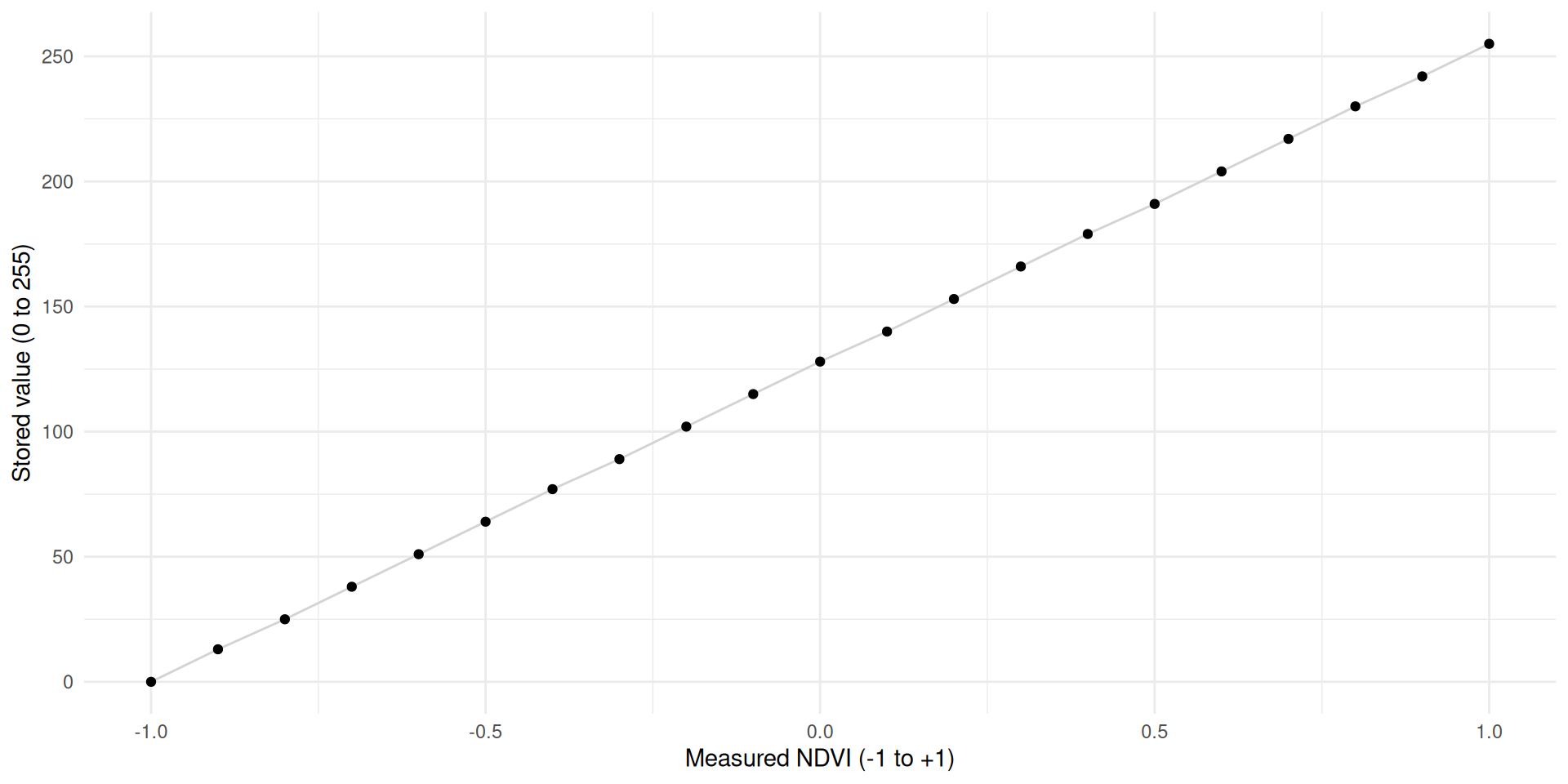
Min-max rescaling

General formula to rescale \(x\) into range \([a, b]\):

\[x' = a + \frac{(x - \min(x))\,(b - a)}{\max(x) - \min(x)}\]

For NDVI (\(x \in [-1,\,1]\), target \([a, b] = [0,\,255]\)):

\[x' = 0 + \frac{(x - (-1))\,\times\,255}{1-(-1)} = \frac{(x+1)\times 255}{2}\]

Simplified:

\[\boxed{x' = 127.5\,x + 127.5}\]

→ e.g. NDVI 0.2 is stored as \(127.5 \times 0.2 + 127.5 = 153\)

• \(a = 0\), \(b = 255\) (Byte range); \(\min(x) = -1\), \(\max(x) = 1\) (NDVI range)
• The two parameters 127.5 and 127.5 are the scale and offset of this linear transform

Precision trade-off

Storing NDVI in Byte limits us to 256 distinct values:

\[\text{precision} = \frac{\max(x) - \min(x)}{b - a} = \frac{1 - (-1)}{255 - 0} \approx 0.0078\]

→ Every stored NDVI is rounded to the nearest 0.0078

For most vegetation mapping applications, NDVI differences below ~0.01 are not ecologically meaningful → Byte precision is usually sufficient

Need finer precision? Use UInt16 (0–65,535): \(\frac{2}{65535} \approx 0.00003\)

R: rescaling vectors

scale_minmax <- function(x, a = 0, b = 255) {
  x_new <- a + (x - min(x)) * (b - a) / (max(x) - min(x))
  round(x_new, 0)
}

measured_ndvi <- seq(-1, 1, 0.1)
stored_value <- scale_minmax(measured_ndvi)

Restoring original values

• The transform \(x' = 127.5\,x + 127.5\) is reversible
• Invert the function to recover originals: \(x = \dfrac{x' - 127.5}{127.5}\)
• More generally: two parameters describe the transform — scale and offset
• Ideally transformation of values is not done within the R / Python session. Best practice:
  • GDAL transforms values during writing
  • GDAL stores scale and offset in the file metadata
  • GDAL restores the original values on read
• However, this is not always the case “in the wild”

• No need to tell your colleague about the transform — it’s in the GeoTIFF metadata
• rast("INT1U.tif") returns the original floating-point values; the Byte storage is invisible

GDAL scale/offset in R

• terra::writeRaster supports scale = and offset = arguments — it transforms on write, inverts on read.
• The user needs to know (calculate) these values beforehand
• The formula to determine scale and offset can be derived by the min-max formula

\[\text{scale} = \frac{b - a}{\max(x) - \min(x)}, \qquad \text{offset} = \frac{a\,\max(x) - b\,\min(x)}{\max(x) - \min(x)}\]

get_scale_offset <- function(x, a = 0, b = 255) {  # x must be a SpatRaster
  library(terra)
3  mm    <- minmax(x)
  min_x <- mm[1, 1]
  max_x <- mm[2, 1]

  list(
1    scale  = (max_x - min_x) / (b - a),
2    offset = min_x - a * (max_x - min_x) / (b - a)
  )
}

1

writeRaster divides by scale: stored = (x − offset) / scale

2

writeRaster subtracts offset; for a = 0 this simplifies to min_x

3

Use the global min/max function, not per-cell (e.g. min())

• min(raster) returns per-cell minimum over bands, NOT the global minimum → always use minmax() or global()
• terra’s writeRaster applies stored = (x - offset) / scale; solving for offset such that min_x maps to a gives offset = min_x - a * scale

Scale / offset in practice

library(terra)

elev <- rast(system.file("ex/elev.tif", package = "terra"))
plot(elev, main = paste(minmax(elev), collapse = " – "))

so <- get_scale_offset(elev)

so

$scale
[1] 1.592157

$offset
[1] 141

# Note: floating-point rounding may introduce NAs at boundary values
writeRaster(elev, "data-out/INT1U.tif", datatype = "INT1U", overwrite = TRUE,
            scale = so$scale, offset = so$offset)

writeRaster(elev, "data-out/FLT4S.tif", datatype = "FLT4S", overwrite = TRUE)

file.size("data-out/INT1U.tif") / file.size("data-out/FLT4S.tif")

[1] 0.6759172

Scale and offset are visible in the file metadata — any GDAL-powered tool can read them:

gdal raster info -f json data-out/INT1U.tif | jq '.bands[] | {scale, offset}'

{
  "scale": 1.592156862745098,
  "offset": 141.0
}

• Reading INT1U.tif back gives original float values — the Byte storage is transparent
• The ratio shows how much smaller the Byte file is compared to Float32 (FLT4S)
• In the gdalinfo output, look for Type=Byte (stored type) and Scale/Offset under Band 1

gdal raster info

Extracting file (meta) data

gdal raster info

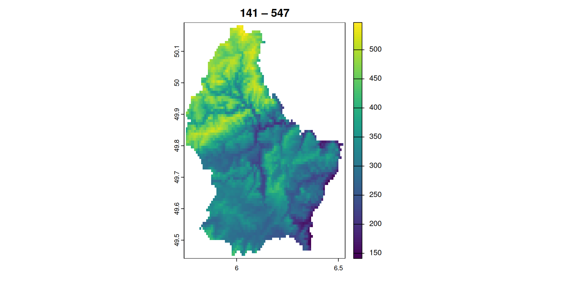
• gdal raster info lists information about a raster dataset
• We’ll use elev-lux.tif — a small elevation model of Luxembourg — as our running example

• List all arguments with --help:

gdal raster info --help

Usage: gdal raster info [OPTIONS] <INPUT>

Return information on a raster dataset.

Positional arguments:
  -i, --dataset, --input <INPUT>                       Input raster dataset [required]

Common Options:
  -h, --help                                           Display help message and exit
  --json-usage                                         Display usage as JSON document and exit
  --config <KEY>=<VALUE>                               Configuration option [may be repeated]

Options:
  -f, --of, --format, --output-format <OUTPUT-FORMAT>  Output format. OUTPUT-FORMAT=json|text (default: json)
  --mm, --min-max                                      Compute minimum and maximum value
  --stats                                              Retrieve or compute statistics, using all pixels
                                                       Mutually exclusive with --approx-stats
  --approx-stats                                       Retrieve or compute statistics, using a subset of pixels
                                                       Mutually exclusive with --stats
  --hist                                               Retrieve or compute histogram

Advanced Options:
  --oo, --open-option <KEY>=<VALUE>                    Open options [may be repeated]
  --if, --input-format <INPUT-FORMAT>                  Input formats [may be repeated]
  --no-gcp                                             Suppress ground control points list printing
  --no-md                                              Suppress metadata printing
  --no-ct                                              Suppress color table printing
  --no-fl                                              Suppress file list printing
  --checksum                                           Compute pixel checksum
  --list-metadata-domains, --list-mdd                  List all metadata domains available for the dataset
  --mdd, --metadata-domain <METADATA-DOMAIN>           Report metadata for the specified domain. 'all' can be used to report metadata in all domains

Esoteric Options:
  --no-nodata                                          Suppress retrieving nodata value
  --no-mask                                            Suppress mask band information
  --subdataset <SUBDATASET>                            Use subdataset of specified index (starting at 1), instead of the source dataset itself

For more details, consult https://gdal.org/programs/gdal_raster_info.html

WARNING: the gdal command is provisionally provided as an alternative interface to GDAL and OGR command line utilities.
The project reserves the right to modify, rename, reorganize, and change the behavior of the utility
until it is officially frozen in a future feature release of GDAL.

• Named args use --flag convention; positional arg is <filename>
• Default output is JSON (text from GDAL 3.12 when run interactively) — use -f json to be explicit

• Get all metadata and display output as text

gdal raster info -f text data/raster-deepdive/elev-lux.tif

Driver: GTiff/GeoTIFF
Files: data/raster-deepdive/elev-lux.tif
       data/raster-deepdive/elev-lux.tif.aux.xml
Size is 95, 90
Coordinate System is:
GEOGCRS["WGS 84",
    ENSEMBLE["World Geodetic System 1984 ensemble",
        MEMBER["World Geodetic System 1984 (Transit)"],
        MEMBER["World Geodetic System 1984 (G730)"],
        MEMBER["World Geodetic System 1984 (G873)"],
        MEMBER["World Geodetic System 1984 (G1150)"],
        MEMBER["World Geodetic System 1984 (G1674)"],
        MEMBER["World Geodetic System 1984 (G1762)"],
        MEMBER["World Geodetic System 1984 (G2139)"],
        MEMBER["World Geodetic System 1984 (G2296)"],
        ELLIPSOID["WGS 84",6378137,298.257223563,
            LENGTHUNIT["metre",1]],
        ENSEMBLEACCURACY[2.0]],
    PRIMEM["Greenwich",0,
        ANGLEUNIT["degree",0.0174532925199433]],
    CS[ellipsoidal,2],
        AXIS["geodetic latitude (Lat)",north,
            ORDER[1],
            ANGLEUNIT["degree",0.0174532925199433]],
        AXIS["geodetic longitude (Lon)",east,
            ORDER[2],
            ANGLEUNIT["degree",0.0174532925199433]],
    USAGE[
        SCOPE["Horizontal component of 3D system."],
        AREA["World."],
        BBOX[-90,-180,90,180]],
    ID["EPSG",4326]]
Data axis to CRS axis mapping: 2,1
Origin = (5.741666666666666,50.191666666666663)
Pixel Size = (0.008333333333333,-0.008333333333333)
Metadata:
  AREA_OR_POINT=Area
Image Structure Metadata:
  COMPRESSION=LZW
  INTERLEAVE=BAND
Corner Coordinates:
Upper Left  (   5.7416667,  50.1916667) (  5d44'30.00"E, 50d11'30.00"N)
Lower Left  (   5.7416667,  49.4416667) (  5d44'30.00"E, 49d26'30.00"N)
Upper Right (   6.5333333,  50.1916667) (  6d32' 0.00"E, 50d11'30.00"N)
Lower Right (   6.5333333,  49.4416667) (  6d32' 0.00"E, 49d26'30.00"N)
Center      (   6.1375000,  49.8166667) (  6d 8'15.00"E, 49d49' 0.00"N)
Band 1 Block=95x43 Type=Int16, ColorInterp=Gray
  Description = elevation
  Min=141.000 Max=547.000 
  Minimum=141.000, Maximum=547.000, Mean=-9999.000, StdDev=-9999.000
  NoData Value=-32768
  Metadata:
    STATISTICS_MINIMUM=141
    STATISTICS_MAXIMUM=547
    STATISTICS_MEAN=-9999
    STATISTICS_STDDEV=-9999

• Output includes: driver, dimensions, CRS, origin, pixel size, bands, datatype, NoData value, scale/offset
• This is the quickest way to inspect any raster file without opening R or Python

• The metadata output format (-f) can either be text or to json
• Where text is more human readable, json is structured and machine readable

gdal raster info -f json data/raster-deepdive/elev-lux.tif

{
  "description":"data/raster-deepdive/elev-lux.tif",
  "driverShortName":"GTiff",
  "driverLongName":"GeoTIFF",
  "files":[
    "data/raster-deepdive/elev-lux.tif",
    "data/raster-deepdive/elev-lux.tif.aux.xml"
  ],
  "size":[
    95,
    90
  ],
  "coordinateSystem":{
    "wkt":"GEOGCRS[\"WGS 84\",\n    ENSEMBLE[\"World Geodetic System 1984 ensemble\",\n        MEMBER[\"World Geodetic System 1984 (Transit)\"],\n        MEMBER[\"World Geodetic System 1984 (G730)\"],\n        MEMBER[\"World Geodetic System 1984 (G873)\"],\n        MEMBER[\"World Geodetic System 1984 (G1150)\"],\n        MEMBER[\"World Geodetic System 1984 (G1674)\"],\n        MEMBER[\"World Geodetic System 1984 (G1762)\"],\n        MEMBER[\"World Geodetic System 1984 (G2139)\"],\n        MEMBER[\"World Geodetic System 1984 (G2296)\"],\n        ELLIPSOID[\"WGS 84\",6378137,298.257223563,\n            LENGTHUNIT[\"metre\",1]],\n        ENSEMBLEACCURACY[2.0]],\n    PRIMEM[\"Greenwich\",0,\n        ANGLEUNIT[\"degree\",0.0174532925199433]],\n    CS[ellipsoidal,2],\n        AXIS[\"geodetic latitude (Lat)\",north,\n            ORDER[1],\n            ANGLEUNIT[\"degree\",0.0174532925199433]],\n        AXIS[\"geodetic longitude (Lon)\",east,\n            ORDER[2],\n            ANGLEUNIT[\"degree\",0.0174532925199433]],\n    USAGE[\n        SCOPE[\"Horizontal component of 3D system.\"],\n        AREA[\"World.\"],\n        BBOX[-90,-180,90,180]],\n    ID[\"EPSG\",4326]]",
    "dataAxisToSRSAxisMapping":[
      2,
      1
    ]
  },
  "geoTransform":[
    5.7416666666666663,
    0.0083333333333333,
    0.0,
    50.1916666666666629,
    0.0,
    -0.0083333333333333
  ],
  "metadata":{
    "":{
      "AREA_OR_POINT":"Area"
    },
    "IMAGE_STRUCTURE":{
      "COMPRESSION":"LZW",
      "INTERLEAVE":"BAND"
    }
  },
  "cornerCoordinates":{
    "upperLeft":[
      5.7416667,
      50.1916667
    ],
    "lowerLeft":[
      5.7416667,
      49.4416667
    ],
    "lowerRight":[
      6.5333333,
      49.4416667
    ],
    "upperRight":[
      6.5333333,
      50.1916667
    ],
    "center":[
      6.1375,
      49.8166667
    ]
  },
  "wgs84Extent":{
    "type":"Polygon",
    "coordinates":[
      [
        [
          5.7416667,
          50.1916667
        ],
        [
          5.7416667,
          49.4416667
        ],
        [
          6.5333333,
          49.4416667
        ],
        [
          6.5333333,
          50.1916667
        ],
        [
          5.7416667,
          50.1916667
        ]
      ]
    ]
  },
  "bands":[
    {
      "band":1,
      "block":[
        95,
        43
      ],
      "type":"Int16",
      "colorInterpretation":"Gray",
      "description":"elevation",
      "min":141.0,
      "max":547.0,
      "minimum":141.0,
      "maximum":547.0,
      "mean":-9999.0,
      "stdDev":-9999.0,
      "noDataValue":-32768,
      "metadata":{
        "":{
          "STATISTICS_MINIMUM":"141",
          "STATISTICS_MAXIMUM":"547",
          "STATISTICS_MEAN":"-9999",
          "STATISTICS_STDDEV":"-9999"
        }
      }
    }
  ],
  "stac":{
    "proj:shape":[
      90,
      95
    ],
    "proj:wkt2":"GEOGCRS[\"WGS 84\",\n    ENSEMBLE[\"World Geodetic System 1984 ensemble\",\n        MEMBER[\"World Geodetic System 1984 (Transit)\"],\n        MEMBER[\"World Geodetic System 1984 (G730)\"],\n        MEMBER[\"World Geodetic System 1984 (G873)\"],\n        MEMBER[\"World Geodetic System 1984 (G1150)\"],\n        MEMBER[\"World Geodetic System 1984 (G1674)\"],\n        MEMBER[\"World Geodetic System 1984 (G1762)\"],\n        MEMBER[\"World Geodetic System 1984 (G2139)\"],\n        MEMBER[\"World Geodetic System 1984 (G2296)\"],\n        ELLIPSOID[\"WGS 84\",6378137,298.257223563,\n            LENGTHUNIT[\"metre\",1]],\n        ENSEMBLEACCURACY[2.0]],\n    PRIMEM[\"Greenwich\",0,\n        ANGLEUNIT[\"degree\",0.0174532925199433]],\n    CS[ellipsoidal,2],\n        AXIS[\"geodetic latitude (Lat)\",north,\n            ORDER[1],\n            ANGLEUNIT[\"degree\",0.0174532925199433]],\n        AXIS[\"geodetic longitude (Lon)\",east,\n            ORDER[2],\n            ANGLEUNIT[\"degree\",0.0174532925199433]],\n    USAGE[\n        SCOPE[\"Horizontal component of 3D system.\"],\n        AREA[\"World.\"],\n        BBOX[-90,-180,90,180]],\n    ID[\"EPSG\",4326]]",
    "proj:epsg":4326,
    "proj:projjson":{
      "$schema":"https://proj.org/schemas/v0.7/projjson.schema.json",
      "type":"GeographicCRS",
      "name":"WGS 84",
      "datum_ensemble":{
        "name":"World Geodetic System 1984 ensemble",
        "members":[
          {
            "name":"World Geodetic System 1984 (Transit)",
            "id":{
              "authority":"EPSG",
              "code":1166
            }
          },
          {
            "name":"World Geodetic System 1984 (G730)",
            "id":{
              "authority":"EPSG",
              "code":1152
            }
          },
          {
            "name":"World Geodetic System 1984 (G873)",
            "id":{
              "authority":"EPSG",
              "code":1153
            }
          },
          {
            "name":"World Geodetic System 1984 (G1150)",
            "id":{
              "authority":"EPSG",
              "code":1154
            }
          },
          {
            "name":"World Geodetic System 1984 (G1674)",
            "id":{
              "authority":"EPSG",
              "code":1155
            }
          },
          {
            "name":"World Geodetic System 1984 (G1762)",
            "id":{
              "authority":"EPSG",
              "code":1156
            }
          },
          {
            "name":"World Geodetic System 1984 (G2139)",
            "id":{
              "authority":"EPSG",
              "code":1309
            }
          },
          {
            "name":"World Geodetic System 1984 (G2296)",
            "id":{
              "authority":"EPSG",
              "code":1383
            }
          }
        ],
        "ellipsoid":{
          "name":"WGS 84",
          "semi_major_axis":6378137,
          "inverse_flattening":298.257223563
        },
        "accuracy":"2.0",
        "id":{
          "authority":"EPSG",
          "code":6326
        }
      },
      "coordinate_system":{
        "subtype":"ellipsoidal",
        "axis":[
          {
            "name":"Geodetic latitude",
            "abbreviation":"Lat",
            "direction":"north",
            "unit":"degree"
          },
          {
            "name":"Geodetic longitude",
            "abbreviation":"Lon",
            "direction":"east",
            "unit":"degree"
          }
        ]
      },
      "scope":"Horizontal component of 3D system.",
      "area":"World.",
      "bbox":{
        "south_latitude":-90,
        "west_longitude":-180,
        "north_latitude":90,
        "east_longitude":180
      },
      "id":{
        "authority":"EPSG",
        "code":4326
      }
    },
    "proj:transform":[
      5.7416666666666663,
      0.0083333333333333,
      0.0,
      50.1916666666666629,
      0.0,
      -0.0083333333333333
    ],
    "raster:bands":[
      {
        "data_type":"int16",
        "stats":{
          "minimum":141.0,
          "maximum":547.0,
          "mean":-9999.0,
          "stddev":-9999.0
        },
        "nodata":-32768
      }
    ],
    "eo:bands":[
      {
        "name":"b1",
        "description":"elevation"
      }
    ]
  }
}

• JSON in turn can be parsed using jq — a lightweight command-line JSON processor
  • Navigates JSON with .key (field access) and [] (array iteration)
  • Install: conda install -c conda-forge jq

gdal raster info -f json data/raster-deepdive/elev-lux.tif | jq ".driverLongName"

"GeoTIFF"

Extract a single field — .bands[] iterates over bands, .min selects the field:

gdal raster info -f json data/raster-deepdive/elev-lux.tif | jq ".bands[].min"

141.0

Extract multiple fields — pipe | into {min, max} to select both at once:

gdal raster info -f json data/raster-deepdive/elev-lux.tif | jq '.bands[] | {min, max}'

{
  "min": 141.0,
  "max": 547.0
}

gdal raster info: terminal histogram

Extract histogram buckets and visualise with bashplotlib:

gdal raster info --hist -f json data/raster-deepdive/elev-lux.tif |
1  jq ".bands[].histogram.buckets[]" |
2  hist -w 1 -p +

1

Extract raw bucket counts from the histogram array

2

hist from bashplotlib

 19|  +
 18|  +
 17|  +
 16|  +
 15|  +
 14|  +
 13|  +
 12|  +    +
 11|  +    +
 10| ++ ++ +
  9| ++ ++++                  + +
  8| +++++++  +               + +
  7| ++++++++ ++++ +    ++    + +
  6| ++++++++ ++++ +   +++    + +
  5| +++++++++++++ +  ++++    + ++ +
  4| ++++++++++++++++ ++++++  + ++ ++     +
  3| +++++++++++++++++++++++ ++ ++ ++   + +  + +         +  +
  2| +++++++++++++++++++++++++++++ ++++ + + ++ + +   +   +  + +
  1| ++++++++++++++++++++++++++++++++++ ++++++++ + +++  +++ +++ + +  +   ++
    ----------------------------------------------------------------------

• Install bashplotlib with pip install bashplotlib
• Useful for quick EDA directly in the terminal without opening R/Python

NoData in rasters

NoData in rasters

• Raster files have no explicit null type — every cell must hold a numeric value
• To mark cells as missing, a two-step approach is used:
  1. Assign a reserved value within the datatype’s range (e.g. the maximum possible value)
  2. Label that value as NoData in the file metadata

→ Any software reading the file interprets that reserved value as missing, not as a real measurement

• This is different from R’s in-memory NA, which is a proper null type
• The reserved value label lives in the metadata, just like scale/offset

NoData & data types

For integer types, the reserved value must fit within the datatype’s range:

Datatype	Common NoData reserved value
Byte	255 (max value)
Int16	−32,768 (min value)
Float321	NaN or −9999

Risk (integer types): if real data happens to contain the reserved value → those cells silently become NoData

• For Byte: using 255 as NoData means you only have 0–254 for real data
• NaN is an unambiguous bit pattern in IEEE 754 — it represents “undefined result” (e.g. 0/0) and is never a valid number
• The silent data-loss risk applies only to integer types; float types with NaN are safe

1. Float types support NaN (as part of the IEEE 754 standard). -9999 sometimes seen in float rasters is a legacy workaround for older software that cannot handle NaN

NoData in terra

Inspect and set the NoData flag:

library(terra)

elev <- rast(system.file("ex/elev.tif", package = "terra"))

NAflag(elev)   # current NoData reserved value

[1] NaN

# Only use 0 - 254, so that 255 is availalable for "NoData"
so <- get_scale_offset(elev, a = 0, b = 254)

# write with an explicit NoData flag
writeRaster(elev, "data-out/elev_naflag.tif", datatype = "INT1U", overwrite = TRUE,
            scale = so$scale, offset = so$offset, NAflag = 255)

# read back — terra interprets 255 as NA automatically
elev_back <- rast("data-out/elev_naflag.tif")
plot(elev_back, colNA = "black")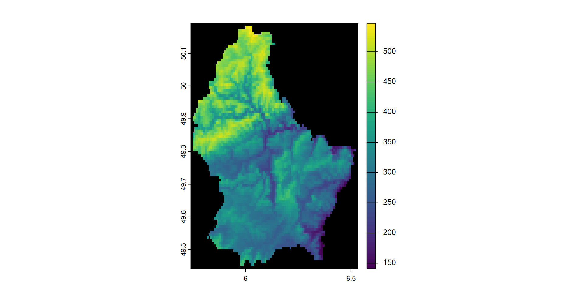

Note that the maximum elevation values are now NA

The reserved value and its NoData label are both visible in the metadata:

gdal raster info -f json data-out/elev_naflag.tif | jq ".bands[].noDataValue"

255

• NAflag() returns the value currently flagged as NoData; NA means no flag is set
• On read, terra converts the flagged value back to R’s NA transparently
• NAflag and datatype are set together in writeRaster — they are two sides of the same coin
• In the gdalinfo output, look for NoData Value=255 under Band 1

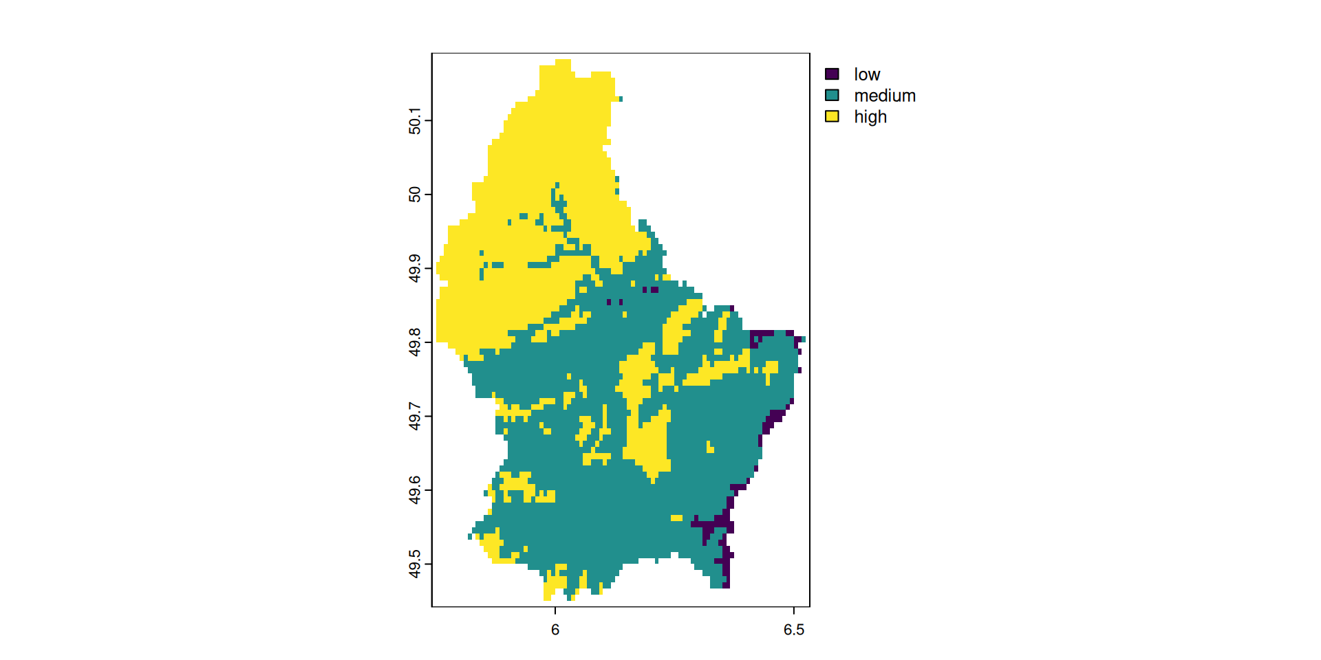
Categorical rasters

Categorical rasters

• Some raster data is categorical, not continuous: land use, soil type, vegetation class, …
• Raster files cannot store text — categories are encoded as integers
• The mapping (integer code → category label) is stored in the file metadata as an attribute table

→ Analogous to R’s factor: an underlying integer + a levels table

→ Choose the smallest integer type that covers the number of categories — Byte handles up to 255 classes

• Most land use / land cover classifications have far fewer than 255 classes → Byte is almost always sufficient
• The attribute table lives in the file metadata, just like scale/offset and NoData flags

Categorical rasters in terra

1elev_cat <- classify(elev, c(0, 200, 350, 550))
2levels(elev_cat) <- data.frame(value = 0:2, label = c("low", "medium", "high"))

plot(elev_cat)

1

Reclassify values into three categories (0-200, 200-350 and 350-550)

2

Relable the default classes to low, medium and high

# write as Byte explicitly (optional, writeRaster makes a reasonable guess)
writeRaster(elev_cat, "data-out/elev_cat.tif", datatype = "INT1U", overwrite = TRUE)

gdal raster info -f json data-out/elev_cat.tif | jq '.bands[].categories[0:3]'

[
  "low",
  "medium",
  "high"
]

• levels() sets the attribute table — same function as for R factors
• cats(elev_cat) to inspect the table after the fact
• On read, terra restores the levels automatically if the attribute table is embedded in the file

Compression

Raster file size

• File size = dimensions × bands × bytes per pixel
• Example: single SRTM tile, one band, Int16 (2 bytes/pixel):

\[3601 \times 3601 \times 2\,\text{B} = 25{,}934{,}402\,\text{B} \approx 25.9\,\text{MB}\]

• Compression reduces storage by exploiting spatial redundancy in pixel values

• Real-world rasters often have large homogeneous regions → high redundancy → compress well
• Redundancy is especially high in categorical rasters (e.g. land cover with few distinct values)

Lossless vs lossy

	Lossless	Lossy
Data preserved?	Perfectly	Approximated
Use case	Scientific data (DEM, multispectral)	Photographic / visual imagery
Examples	LZW, DEFLATE, ZSTD, PACKBITS	JPEG2000, WEBP

→ For scientific analysis always use lossless — lossy compression permanently alters pixel values

• WEBP supports both lossy and lossless modes depending on settings
• Once lossy-compressed, original values cannot be recovered — important for analysis reproducibility
• Much of this section is based on Gandhi (2020) and Paul Ramsey’s GeoTIFF compression guide

How compression works

Exploit repeated values — store each unique value once, track its positions:

Original	100, 101, 102, 100, 100
Compressed	100 → positions [0, 3, 4] 101 → positions [1] 102 → positions [2]

→ 5 values encoded as 3 unique values + a position list

Works best when data contains many repeated or near-repeated values (flat terrain, uniform land cover)

• This is a simplified illustration of dictionary / run-length encoding
• LZW and DEFLATE use more sophisticated variants of this principle

PREDICTOR

LZW, DEFLATE, and ZSTD can use a predictor to improve compression further:

→ Store differences between consecutive values instead of absolute values

Original	100	101	102	100	100
With predictor	100	+1	+1	−2	0

Small differences compress better than large absolute values

Option	Use for
PREDICTOR=1	No predictor (default)
PREDICTOR=2	Integer data (e.g. DEMs)
PREDICTOR=3	Float data

• Predictor=2 works well for integer rasters with gradual spatial variation
• Predictor=3 for float rasters
• Using the wrong predictor (e.g. =3 on integer data) still works but may not compress as well

Tiling & compression costs

• By default, GeoTIFF stores data line by line (strip layout)
• TILED=YES stores data in 256 × 256 pixel blocks

→ Tiling improves random-access reads and is essential for Cloud-Optimized GeoTIFF (COG)

Compression is not free:

• Adds CPU overhead on write and read
• Good default for most scientific workflows: DEFLATE + TILED=YES

• Strip layout is fast for sequential top-to-bottom reads but slow for spatial queries on large files
• ZSTD generally offers better ratios than DEFLATE but has less universal software support
• COG = Cloud-Optimized GeoTIFF; tiling + overviews enable efficient streaming from cloud storage

gdal raster convert

gdal raster convert converts raster files between formats and applies compression:

gdal raster convert --help

Usage: gdal raster convert [OPTIONS] <INPUT> <OUTPUT>

Convert a raster dataset.

Positional arguments:
  -i, --input <INPUT>                                  Input raster dataset [required]
  -o, --output <OUTPUT>                                Output raster dataset (created by algorithm) [required]

Common Options:
  -h, --help                                           Display help message and exit
  --json-usage                                         Display usage as JSON document and exit
  --config <KEY>=<VALUE>                               Configuration option [may be repeated]
  --progress                                           Display progress bar

Options:
  -f, --of, --format, --output-format <OUTPUT-FORMAT>  Output format
  --co, --creation-option <KEY>=<VALUE>                Creation option [may be repeated]
  --overwrite                                          Whether overwriting existing output is allowed
                                                       Mutually exclusive with --append
  --append                                             Append as a subdataset to existing output
                                                       Mutually exclusive with --overwrite

Advanced Options:
  --oo, --open-option <KEY>=<VALUE>                    Open options [may be repeated]
  --if, --input-format <INPUT-FORMAT>                  Input formats [may be repeated]

For more details, consult https://gdal.org/programs/gdal_raster_convert.html

WARNING: the gdal command is provisionally provided as an alternative interface to GDAL and OGR command line utilities.
The project reserves the right to modify, rename, reorganize, and change the behavior of the utility
until it is officially frozen in a future feature release of GDAL.

Key points:

• Two positional arguments: <input_file> <output_file>
• Compression via --co KEY=VALUE (creation options)
• Options are format-specific — always check --help

• Mutually exclusive options are shown as [[-strict]|[-not_strict]] in the help output

gdal raster convert: baseline

gdal raster convert data/raster-deepdive/dhm25_grid_raster.asc data-out/dhm25.tif

File	Size (MB)	Difference
Original (ASCII)	824.43	0 %
GeoTIFF, no compression	535.91	-35 %

gdal raster convert: + DEFLATE

gdal raster convert data/raster-deepdive/dhm25_grid_raster.asc data-out/dhm25_2.tif \
  --co COMPRESS=DEFLATE

File	Size (MB)	Difference
Original (ASCII)	824.43	0 %
GeoTIFF, no compression	535.91	-35 %
COMPRESS=DEFLATE	208.24	-75 %

gdal raster convert: + TILED

gdal raster convert data/raster-deepdive/dhm25_grid_raster.asc data-out/dhm25_3.tif \
  --co COMPRESS=DEFLATE \
  --co TILED=YES

File	Size (MB)	Difference
Original (ASCII)	824.43	0 %
GeoTIFF, no compression	535.91	-35 %
COMPRESS=DEFLATE	208.24	-75 %
TILED=YES	177.50	-78 %

gdal raster convert: + PREDICTOR

gdal raster convert data/raster-deepdive/dhm25_grid_raster.asc data-out/dhm25_4.tif \
  --co COMPRESS=DEFLATE \
  --co TILED=YES \
  --co PREDICTOR=3

File	Size (MB)	Difference
Original (ASCII)	824.43	0 %
GeoTIFF, no compression	535.91	-35 %
COMPRESS=DEFLATE	208.24	-75 %
TILED=YES	177.50	-78 %
PREDICTOR=3	150.89	-82 %

• PREDICTOR=3 for floating-point data; use PREDICTOR=2 for integer data
• Each row in the table adds one -co flag — the cumulative effect shows how the options interact

gdal raster reproject

gdal raster info: get CRS

To reproject a raster, we need to know the source CRS. Is this information available?

gdal raster info -f json data/raster-deepdive/dhm25_grid_raster.asc | \
  jq ".coordinateSystem"

null

→ No CRS — consult the data provider: DHM25 uses LV03/LN02 = EPSG:21781

Confirm via corner coordinates:

gdal raster info -f json data/raster-deepdive/dhm25_grid_raster.asc  | \
  jq ".cornerCoordinates | {upperLeft, lowerRight}"

{
  "upperLeft": [
    479987.5,
    302012.5
  ],
  "lowerRight": [
    865012.5,
    73987.5
  ]
}

• Large x/y values (e.g. 480000, 70000) are characteristic of Swiss LV03 coordinates → confirms EPSG:21781
• If the CRS field is null, the corner coordinates often reveal the projection — know your coordinate ranges

gdal raster reproject

• gdal raster reproject reprojects and transforms raster data
• Two positional arguments: <input> and <output>

gdal raster reproject --help

Usage: gdal raster reproject [OPTIONS] <INPUT> <OUTPUT>

Reproject a raster dataset.

Positional arguments:
  -i, --input <INPUT>                                  Input raster dataset [required]
  -o, --output <OUTPUT>                                Output raster dataset [required]

Common Options:
  -h, --help                                           Display help message and exit
  --json-usage                                         Display usage as JSON document and exit
  --config <KEY>=<VALUE>                               Configuration option [may be repeated]
  --progress                                           Display progress bar

Options:
  -f, --of, --format, --output-format <OUTPUT-FORMAT>  Output format ("GDALG" allowed)
  --co, --creation-option <KEY>=<VALUE>                Creation option [may be repeated]
  --overwrite                                          Whether overwriting existing output is allowed
  -s, --src-crs <SRC-CRS>                              Source CRS
  -d, --dst-crs <DST-CRS>                              Destination CRS
  -r, --resampling <RESAMPLING>                        Resampling method. RESAMPLING=nearest|bilinear|cubic|cubicspline|lanczos|average|rms|mode|min|max|med|q1|q3|sum (default: nearest)
  --resolution <xres>,<yres>                           Target resolution (in destination CRS units)
                                                       Mutually exclusive with --size
  --size <width>,<height>                              Target size in pixels
                                                       Mutually exclusive with --resolution
  --bbox <BBOX>                                        Target bounding box (in destination CRS units)
  --bbox-crs <BBOX-CRS>                                CRS of target bounding box

Advanced Options:
  --if, --input-format <INPUT-FORMAT>                  Input formats [may be repeated]
  --oo, --open-option <KEY>=<VALUE>                    Open options [may be repeated]
  --target-aligned-pixels                              Round target extent to target resolution
  --src-nodata <SRC-NODATA>                            Set nodata values for input bands ('None' to unset). [1.. values]
  --dst-nodata <DST-NODATA>                            Set nodata values for output bands ('None' to unset). [1.. values]
  --add-alpha                                          Adds an alpha mask band to the destination when the source raster have none.
  --wo, --warp-option <NAME>=<VALUE>                   Warping option(s) [may be repeated]
  --to, --transform-option <NAME>=<VALUE>              Transform option(s) [may be repeated]
  --et, --error-threshold <ERROR-THRESHOLD>            Error threshold

For more details, consult https://gdal.org/programs/gdal_raster_reproject.html

WARNING: the gdal command is provisionally provided as an alternative interface to GDAL and OGR command line utilities.
The project reserves the right to modify, rename, reorganize, and change the behavior of the utility
until it is officially frozen in a future feature release of GDAL.

• gdal raster reproject can also resample — reprojection is its primary use case
• Key flags: --src-crs (source CRS), --dst-crs (target CRS), --resampling (resampling method)

gdal raster reproject: reproject

DHM25 has no embedded CRS → specify source and target explicitly:

gdal raster reproject \
  --src-crs EPSG:21781 \
  --dst-crs EPSG:2056 \
  data/raster-deepdive/dhm25_grid_raster.asc \
  data-out/dhm25.tif

0...10...20...30...40...50...60...70...80...90...100 - done.

• EPSG:21781 = old Swiss coordinate system (LV03 / CH1903)
• EPSG:2056 = new Swiss coordinate system (LV95 / CH1903+)
• Output as GeoTIFF — unlike ASC, it supports embedded CRS metadata

gdal raster reproject: verify

Compare before and after — coordinates should shift from LV03 to LV95 range:

gdal raster info -f json data-out/dhm25.tif | \
  jq '.stac."proj:epsg"'

2056

gdal raster info -f json data-out/dhm25.tif | \
  jq ".cornerCoordinates | {upperLeft, lowerRight}"

{
  "upperLeft": [
    2479987.5,
    1302012.5
  ],
  "lowerRight": [
    2865012.5,
    1073987.5
  ]
}

• Corner coordinates in LV95: easting ~2.6M, northing ~1.2M (vs ~480k, ~70k in LV03)
• .coordinateSystem.wkt gives the full CRS definition — look for EPSG:2056 to confirm
• Comparing the corner coordinates to the earlier ASC output is the most intuitive check

Bringing it all together

Three tools, one goal

All three strategies reduce on-disk file size — but they work at different levels:

Tool	Targets	Mechanism
Datatype	Per-pixel cost	1 byte (Byte) vs 4 bytes (Float32)
Scale / offset	Value range	Rescale floats to fit a smaller integer type
Compression	Spatial redundancy	Exploit repeated values across pixels

→ They are complementary — apply all three for maximum effect

→ Order matters: choose datatype first, then compress

• Getting the datatype wrong means you compress a larger file to begin with
• Scale/offset is what makes integer types viable for continuous data — without it you’d lose the value range
• Compression then removes the spatial redundancy that remains regardless of datatype

Practical checklist

When writing a raster to disk:

1. What is my value range? → choose the smallest datatype that fits
2. Can I rescale to fit an integer type? → use scale / offset in writeRaster
3. Are there missing cells? → set NAflag (integer types) or use NaN (float types)
4. Apply lossless compression: COMPRESS=DEFLATE + TILED=YES
   • Add PREDICTOR=2 for integer data, PREDICTOR=3 for float data

Default recommendation for most scientific rasters:

INT1U / Int16  +  scale/offset  +  DEFLATE  +  TILED=YES  +  PREDICTOR=2

• For data that genuinely needs float precision (e.g. model outputs with many significant digits), skip the scale/offset step and use FLT4S + DEFLATE + TILED + PREDICTOR=3
• ZSTD can replace DEFLATE for better ratios where broad software compatibility is less critical

References

Amatulli, Giuseppe. 2024. Geocomputation and Machine Learning for Environmental Applications. Http://spatial-ecology.net/docs/build/html/GDAL/gdal_osgeo.html.

Gandhi, Ujaval. 2020. Mastering GDAL Tools (Full Course). Https://courses.spatialthoughts.com/gdal-tools.html#compressing-output.